Automation’s current challenge: Finding opportunity in obsolescence

It is no secret that many of our control systems are reaching their twilight years. For some, they are already there. According to one report, there are currently $65 billion worth of obsolete control systems worldwide, and that number is increasing every day.

This is especially true in oil and gas, a sector that is quickly outgrowing the various upgrades and modifications that have been made to its aging sys­tems over the years. But the term “upgrades” is a misnomer here, as the intention is simply to main­tain—not improve—basic operational functionality. These manufacturers continue to refurbish obsolete systems with the hope of squeezing another year or two out of them. Though the goal is cost sav­ings, ultimately this approach is the least efficient and most costly. Significant downtime is inevitable when the system completely breaks down.

But breakdowns are not the only concern. Ob­solescence is. With the ever-increasing velocity of change in manufacturing, it is becoming more and more clear that the old way is no longer the only path forward. In fact, it is a dead end. To keep up with the evolving automation landscape, we have to approach obsolescence as an oppor­tunity for operational improvement and cost re­duction. An opportunity to innovate rather than replicate. An opportunity for American manufac­turers to regain their competitive edge.

Different approaches to DCS and PLC migration

When a control system begins to outlive its use-fullness, isolating failed parts and replacing them with new ones is a common approach. But begins as required maintenance quickly becomes overextension. Systems running above their design capacity reduce operational efficiency. This means the cost savings from replacing a part rather than the entire system are not just nullified; they are actually reversed. You might think you are saving money, but you are actually losing more of it than you think due to production inefficiencies.

Fully leverage and innovate

Proactive manufacturers do not wait for process downtime to force their hand. They have migra­tion strategies in place before the system begins to lag. They bring in outside vendors to demonstrate new technology and systems integrators for unbi­ased support and expertise. They conduct front-end loading (FEL) studies to identify opportunities for improvement. They do not just look to get by; they look to get ahead.

Make the most of this opportunity Perhaps you have already begun to consider mi­grating your distributed control system (DCS) or programmable logic controller (PLC) system. Or perhaps your system is on its last leg, and you are worried about downtime once it fails completely. Either way, if you want to remain competitive—or regain your competitive edge—waiting is not an option in today’s manufacturing landscape.

Conduct FEL studies to determine how efficien­cies built into your new system can help you re-coup the costs of migration sooner than you think. Take what you learn to make a case for the capital you will need to move forward. Collaborate with systems integration experts to determine the best path forward. And, above all, start today

Part 1: The basic concepts and proportional control.

Most process control engineers have been exposed to the basic equation in a form that looks something like this:

More than you want to swallow in one bite? Let’s break this down into the major components:

Output: u(t)  is the output of the controller at the end of the scan. If the output of the controller is a valve, then the output is the valve position that the controller is requesting after it has seen the inputs. In most controllers, this is actually the change in output from 50%. So if u(t) = 0 then the valve output is 50%; if u(t) = 1 then the valve output is 51%; and if u(t) = -2 then the valve output is 48%. You get the idea. But what’s important is that it’s not a change in output from the previous scan, but a new output.

Proportional
K_pe(t) is the proportional component, the P in PID. If you have a controller configured as proportional only, this is it. So let’s look at how this works.

Let’s start with my own misconception of how I thought it worked. When I imagine a controller, I picture myself turning a valve while watching a gage. I look at the gage, decide if I need more or less, turn that valve a little more or a little less, and then repeat the process until the gage shows the value I want. That sounds fundamentally logical, but it is not how a proportional only controller works. It’s more like if I were to look at the gage, subtract what it reads from what I want it to read, and then take that error over to a chart to look up a new value for the valve.

e(t) usually called error, is simply the difference between the setpoint and the process variable. It is the difference between where you are and where you want to be, right now, at this instant.

K_p gain, is a factor that is multiplied by the error to give you the new output, the new valve position. It’s that simple. The error at that instant of the scan is calculated and the new output is calculated.

Let’s look at an example of pseudo code to explore how this works:

Error = Setpoint - ProcessValue;
Output = K * Error;
This control algorithm is deceptively simple, yet it gives an immediate response to a setpoint change or a disturbance in the process. And if K is set correctly, will quickly move the process toward the setpoint. But, it won’t get the process to the setpoint because there has to be some error if the output is anything other than 50%.

Note: On some systems (though not often in modern systems), gain is expressed as proportional band. Proportional band is defined as the amount of change in the controlled variable required to drive the loop output from 0 to 100%. To convert between the two, gain = 100/PB.

Tuning PID control loops for fast response

When choosing a tuning strategy for a specific control loop, it is important to match the technique to the needs of that loop and the larger process. It is also important to have more than one approach in your repertoire, and the Cohen-Coon method can be a handy addition in the right situation.

The well-known Ziegler-Nichols tuning rules work well only on processes with very long time constants relative to their dead times, and on level control loops. However, its performance is not good on flow, liquid pressure, and many other loops that require fast adjustment. In contrast, the Cohen-Coon tuning rules work well on virtually all self-regulating processes and were designed to give a very fast response.

The method's original design resulted in loops with too much oscillatory response and consequently fell into disuse. However, with some modification, Cohen-Coon tuning rules proved their value for control loops that need to respond quickly while being much less prone to oscillations.

Applicable process types

The Cohen-Coon tuning method isn't suitable for every application. For starters, it can be used only on self-regulating processes. Most control loops, e.g., flow, temperature, pressure, speed, and composition, are, at least to some extent, self-regulating processes. (On the other hand, the most common integrating process is a level control loop.)

A self-regulating process always stabilizes at some point of equilibrium, which depends on the process design and the controller output. If the controller output is set to a different value, the process will respond and stabilize at a new point of equilibrium.

Target controller algorithm

Cohen-Coon tuning rules have been designed for use on a non-interactive controller algorithm such as that provided by the Dataforth MAQ 20 industrial data acquisition and control system. There are controllers with similar characteristics available from other suppliers.

Procedure

To apply modified Cohen-Coon tuning rules, follow the steps below. The process variable and controller output must be time-trended so that measurements can be taken from them.

1. Do a controller output step test:

• Put the controller in manual and wait for the process to settle out.
• Make a step change in the CO (controller output) of a few percent and wait for the PV (process variable) to settle out. The size of this step should be large enough that the PV moves well clear of the process noise and disturbance level. A total movement of five times more than the peak-to-peak level of the noise and disturbances on the PV should be sufficient.

2. Determine the process characteristics (see Figure 1):

• If the PV is not ranged 0-100%, convert the change in PV to a percentage of the range: change in PV [in %] = change in PV [in engineering units] × 100 / (PV upper calibration limit - PV lower calibration limit).
• Calculate the process gain (g_p): g_p = total change in PV [in %] / change in CO [in %].
• Find the maximum slope of the PV response curve. This will be at the point of inflection. Draw a tangential line through the PV response curve at this point.
• Extend this line to intersect with the original level of the PV before the step in CO.
• Take note of the time value at this intersection and calculate the dead time (t_d): t_d = time difference between the change in CO and the intersection of the tangential line and the original PV level.
• If t_d was measured in seconds, divide it by 60 to convert it to minutes. (Since the Dataforth PID controller uses minutes as its time base for integral time, all measurements have to be made in minutes or converted to minutes. Many other controllers are similar.)
• Calculate the value of the PV at 63% of its total change.
• On the PV reaction curve, find the time value at which the PV reaches this level.
• Calculate the time constant (t): t = time difference between intersection at the end of dead time and the PV reaching 63% of its total change.
• If t was measured in seconds, divide it by 60 to convert it to minutes.

3. Repeat steps 1 and 2 three more times to obtain good average values for the process characteristics.

4. Calculate controller settings for a PI or PID controller using the modified Cohen-Coon equations below. (The modified rules calculate the controller gain as ½ of that calculated by the original rules.) 

5. Enter the values into the controller, make sure the algorithm is set to non-interactive, and put the controller in automatic mode.

6. Change the setpoint to test the new values.

Do fine tuning if necessary. The control loop's response can be slowed down and made less oscillatory, if needed, by decreasing K_C and/or increasing T_I.

Conclusion

These modified Cohen-Coon tuning rules are an excellent method for achieving fast response on virtually all control loops with self-regulating processes. They are an effective and highly reliable alternative to the Ziegler-Nichols tuning method, which does not work well when applied to many self-regulating processes.

The Future of Industrial Automation

Since the turn of the century, the global recession has affected most businesses, including industrial automation. After four years of the new millennium, here are my views on the directions in which the automation industry is moving.

The rear-view mirror

Because of the relatively small production volumes and huge varieties of applications, industrial automation typically utilizes new technologies developed in other markets. Automation companies tend to customize products for specific applications and requirements. So the innovation comes from targeted applications, rather than any hot, new technology.

Over the past few decades, some innovations have indeed given industrial automation new surges of growth: The programmable logic controller (PLC) – developed by Dick Morley and others – was designed to replace relay-logic; it generated growth in applications where custom logic was difficult to implement and change. The PLC was a lot more reliable than relay-contacts, and much easier to program and reprogram. Growth was rapid in automobile test-installations, which had to be re-programmed often for new car models. The PLC has had a long and productive life – some three decades – and (understandably) has now become a commodity.

At about the same time that the PLC was developed, another surge of innovation came through the use of computers for control systems. Mini-computers replaced large central mainframes in central control rooms, and gave rise to "distributed" control systems (DCS), pioneered by Honeywell with its TDC 2000. But, these were not really "distributed" because they were still relatively large clumps of computer hardware and cabinets filled with I/O connections.

The arrival of the PC brought low-cost PC-based hardware and software, which provided DCS functionality with significantly reduced cost and complexity. There was no fundamental technology innovation here—rather, these were innovative extensions of technology developed for other mass markets, modified and adapted for industrial automation requirements.

On the sensor side were indeed some significant innovations and developments which generated good growth for specific companies. With better specifications and good marketing, Rosemount's differential pressure flow-sensor quickly displaced lesser products. And there were a host of other smaller technology developments that caused pockets of growth for some companies. But few grew beyond a few hundred million dollars in annual revenue.

Automation software has had its day, and can't go much further. No "inflection point" here. In the future, software will embed within products and systems, with no major independent innovation on the horizon. The plethora of manufacturing software solutions and services will yield significant results, but all as part of other systems.

So, in general, innovation and technology can and will reestablish growth in industrial automation. But, there won't be any technology innovations that will generate the next Cisco or Apple or Microsoft.

We cannot figure out future trends merely by extending past trends; it’s like trying to drive by looking only at a rear-view mirror. The automation industry does NOT extrapolate to smaller and cheaper PLCs, DCSs, and supervisory control and data acquisition systems; those functions will simply be embedded in hardware and software. Instead, future growth will come from totally new directions.

New technology directions

Industrial automation can and will generate explosive growth with technology related to new inflection points: nanotechnology and nanoscale assembly systems; MEMS and nanotech sensors (tiny, low-power, low-cost sensors) which can measure everything and anything; and the pervasive Internet, machine to machine (M2M) networking.

Real-time systems will give way to complex adaptive systems and multi-processing. The future belongs to nanotech, wireless everything, and complex adaptive systems.

Major new software applications will be in wireless sensors and distributed peer-to-peer networks – tiny operating systems in wireless sensor nodes, and the software that allows nodes to communicate with each other as a larger complex adaptive system. That is the wave of the future.

The fully-automated factory

Automated factories and processes are too expensive to be rebuilt for every modification and design change – so they have to be highly configurable and flexible. To successfully reconfigure an entire production line or process requires direct access to most of its control elements – switches, valves, motors and drives – down to a fine level of detail.

The vision of fully automated factories has already existed for some time now: customers order online, with electronic transactions that negotiate batch size (in some cases as low as one), price, size and color; intelligent robots and sophisticated machines smoothly and rapidly fabricate a variety of customized products on demand.

The promise of remote-controlled automation is finally making headway in manufacturing settings and maintenance applications. The decades-old machine-based vision of automation – powerful super-robots without people to tend them – underestimated the importance of communications. But today, this is purely a matter of networked intelligence which is now well developed and widely available.

Communications support of a very high order is now available for automated processes: lots of sensors, very fast networks, quality diagnostic software and flexible interfaces – all with high levels of reliability and pervasive access to hierarchical diagnosis and error-correction advisories through centralized operations.

The large, centralized production plant is a thing of the past. The factory of the future will be small, movable (to where the resources are, and where the customers are). For example, there is really no need to transport raw materials long distances to a plant, for processing, and then transport the resulting product long distances to the consumer. In the old days, this was done because of the localized know-how and investments in equipment, technology and personnel. Today, those things are available globally.

Hard truths about globalization

The assumption has always been that the US and other industrialized nations will keep leading in knowledge-intensive industries while developing nations focus on lower skills and lower labor costs. That's now changed. The impact of the wholesale entry of 2.5 billion people (China and India) into the global economy will bring big new challenges and amazing opportunities.

Beyond just labor, many businesses (including major automation companies) are also outsourcing knowledge work such as design and engineering services. This trend has already become significant, causing joblessness not only for manufacturing labor, but also for traditionally high-paying engineering positions.

Innovation is the true source of value, and that is in danger of being dissipated – sacrificed to a short-term search for profit, the capitalistic quarterly profits syndrome. Countries like Japan and Germany will tend to benefit from their longer-term business perspectives. But, significant competition is coming from many rapidly developing countries with expanding technology prowess. So, marketing speed and business agility will be offsetting advantages.

The winning differences

In a global market, there are three keys that constitute the winning edge:

• Proprietary products: developed quickly and inexpensively (and perhaps globally), with a continuous stream of upgrade and adaptation to maintain leadership.
• High-value-added products: proprietary products and knowledge offered through effective global service providers, tailored to specific customer needs.
• Global yet local services: the special needs and custom requirements of remote customers must be handled locally, giving them the feeling of partnership and proximity.

To implementing these directions demands management and leadership abilities that are different from old, financially-driven models. In the global economy, automation companies have little choice – they must find more ways and means to expand globally. To do this they need to minimize domination of central corporate cultures, and maximize responsiveness to local customer needs. Multi-cultural countries, like the U.S., will have significant advantages in these important business aspects.

In the new and different business environment of the 21st century, the companies that can adapt, innovate and utilize global resources will generate significant growth and success.

4 Big Trends that Impact Industrial Automation and What To Do About Them, Part 1 of 2

Every decade has its big manufacturing trends and hyped-up IT issue(s). Remember Y2K? Nowadays there are several topics that have been the subject of numerous articles in manufacturing trade publications. These include:

1. The Internet of Things (IoT)
2. Big Data
3. Cloud Computing
4. Industry 4.0.

All of these trends involve a lot of devices networked together and a lot of data available to do things. They also include deciding whether data is stored and applications accessed from the computer next to you or from a server located somewhere else.

The good news is: The supporting technologies behind all the buzzwords are already available. Are they empty hype, a valid threat, or an opportunity? (the answer is yes). In this article, I’ll tackle each of these topics one by one, focusing on what you need to know to sort out reality and react to each.

1. Connected Industrial Devices aka the Internet of Things (IoT)

The IoT is about a lot of industrial devices networked together. For example, I’ve encountered automotive plants with 8,000 devices on a single network and consumer products plants with 12,000.

The benefits of networking these devices include:

• Managing everything from anywhere.
• Reducing complexity and hardware costs with one network technology.
• Moving control and information at will.
• Expanding it all easily.
  

The Internet of Things (IoT) is about connecting industrial devices together and taking advantage of the connectivity for business improvement.

The IoT ChallengeThe challenge is in learning the new technology and understanding how to carefully design for systems that dwarf even the largest fieldbuses.

As the IoT concept continues to develop, vendors and standards groups will take care of the hard stuff. The technology will evolve to accommodate the growth—more wireless will be added, everything will be made more secure, higher levels of network traffic will get managed, and more IP addresses will be created.

When all is said and done, you’ll be able to continue as before, just with a few more zeroes in the number of devices on your network.

The IoT OpportunityUltimately, however, it will be up to you to decide how your company can operate differently when virtually anything can be on your network.

2. The Next Frontier of Manufacturing IT: Big Data

Big Data is about having a ton of information to use. Ten years ago, manufacturers recognized they could and should store production data and, in response, they added storage space at an alarmingly fast rate.

The Big Data ChallengeNow that all this data is at hand, more than one manufacturer has been known to say: “We’re collecting everything, but we aren’t really using any of it; and we aren’t sure what we should do with it all.”

This trend continues today, but with software that knows how to analyze and help you use that data. Some of the best technology is derived from search engine and web companies, like Google and Amazon that measure, interpret and record every twitch their users make. Vendors will continue to make data transport and storage bigger and faster, and will keep creating software to help you use the data.

The challenge with Big Data is how to use it to gain efficiencies, insight speed and competitive advantage.

The Big Data OpportunityYour decision is how to connect the information “gold” in your hands to your company’s business challenges to see new opportunities to gain efficiencies, insight, speed and competitive advantage.

3. Cloud Computing

Cloud computing is about storing your information and computing power somewhere other than the computer next to you. Today, most see cloud computing as an opportunity to gain more computing power and storage space, while reducing the overall cost of maintaining and managing IT equipment and software. They also see new ways to collaborate with others.

While the computing aspect of cloud computing has a ways to go to become truly viable for the industrial space, storage is coming on strong as an easy way to back up and share data.

The Cloud Computing ChallengeLike the IoT and Big Data, vendors will handle the technology issues here as well. Your job is to assess the benefits and risks of having your critical data available and secure when it is located and managed by someone else, somewhere else.

In the industrial world, we define “real-time” and “mission-critical” different than the IT group, so our comfort level with what and how the cloud can work for us may vary dramatically. Proceed here with caution.

The Cloud Computing OpportunityOnce satisfied, however, you can determine how your company might benefit by having virtually unlimited computing power, storage and, eventually, new avenues of collaboration.

4. Industry 4.0

Industry 4.0/Manufacturing 4.0, which originated in Germany, is about the strategic use of smart devices. As a frame of reference, consider this:

• In the 1990s, a photo eye was available that held more than 30 pieces of information when networked on DeviceNet.
• About the same time, variable frequency drives (VFDs) and motor starters went from having only a few analog and digital signals tied in with their power to sharing hundreds of pieces of information when networked.

The point here is that the technology behind Industry 4.0 isn’t new.

The Industry 4.0 Opportunity and ChallengeThe new opportunity with Industry 4.0 is using the wealth of information available from smart, networked devices to revolutionize industrial processes.

The challenge is to think big and drive the change necessary within your organization to capitalize on information available today to for success tomorrow.

Poised to Take AdvantageGiven that the supporting technologies behind all these futuristic industry concepts are available today, the question is: Are you ready to take advantage of them?

In part 2 of this series I will address the steps you need to take to take advantage of these 4 big trends. I will also present some ideas of how these trends might be used by forward thinking organizations.

What do you think of Big Data or the Internet of Things? Is your organization examining how to use them for competitive advantages? I look forward to hearing your thoughts.

How To Make 4-20 mA Current Loop Measurements

It seems that at least one 4-20 mA (milliamp) measurement is required by our typical customer, and the way to do it is a constant source of confusion for many. So I thought I’d zero in on the various 4-20 mA current loop configurations and elaborate on the specifics that  you need to know to make a successful measurement. The following discussion is ordered from the most to least common configuration, and I hope to cover all those that I have encountered in customer applications. If yours isn’t included, please use the comments section to fill me in.

4-20 mA Current Loop Basics

Sensors or other devices with a 4-20 mA current loop output are extremely common in industrial measurement and control applications. They are easy to deploy, have wide power supply requirements, generate a low noise output, and can be transmitted without loss over great distances. We encounter them all the time in both process control and basic measurement data logger and data acquisition applications.

The idea behind 4-20 mA current loop operation is that the sensor draws current from its power source in direct proportion to the mechanical property it measures. Take the example of a 100 psi sensor with a current loop output. With 0 psi applied, the sensor draws 4 mA from its power source. With 100 psi applied the sensor draws 20 mA. At 50 psi the sensor draws 12 mA and so on. The relationship of mechanical property measurement to current output is almost always linear, allowing the resulting current loop data to be scaled with a simple mx+b formula to reveal more useful measurements scaled into engineering units.

How you actually measure the 4-20 mA current loop signal is a function of the sensor’s architecture and the capabilities of the instrument you’ll use for the measurement.

Terminology

So that my discussion translates well across the various kinds of 4-20 mA current loop configurations, I’ve opted to standardize the terminology I use to describe each. Here’s an overview:

“E” (dc excitation)

Most configurations that follow will show a DC voltage excitation source that I denote as “E”. Many who use current loop sensors for the first time are surprised to learn that they need to supply this excitation source. Nonetheless, unless the sensor is self-powered (i.e. AC line powered) an external dc source is required. The good news is that this can sometimes be supplied by the instrument, and the range of acceptable values is usually very wide, typically 10-24 V dc.

“R” (shunt resistor)

Here’s a bit of trivia for you: No instruments measure current directly. They all do it indirectly by measuring the voltage dropped across a resistor of known value, and then they use Ohm’s Law to calculate actual current. The resistor is referred to as a “shunt”, is absolutely required to make a current measurement, and is either supplied externally to, or built into the measuring instrument. For clarity, I assume that it’s supplied externally.

“i” (current loop value ranging from 4-20 mA)

This is the 4-20 mA current signal generated by the sensor. Note that some sensors may draw 0-20 mA and even other values, but the vast majority of them use the 4-20 mA convention.

“v” (shunt voltage that’s proportional to current)

This is the voltage actually measured by the instrument. Since our industry has standardized on a shunt value of 250 Ohms, “v” will range between 1 and 5 volts for a 4-20 mA current loop signal (v=i * resistance). Note that shunt resistor value is arbitrary as long as it’s known. You also need to ensure that it doesn’t burden the loop, so lower values are better than higher. Yes, I mean lower. Remember that we’re working with current, not voltage, so the rules are inverted. Just as infinitely-high resistor loads work well for a voltage source, you can take the load all the way to zero Ohms for a current source without consequence.

 Self-powered Sensors

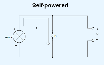
I promised to order these configurations from most to least common, and the self-powered sensor just noses out the first runner up. Self-powered sensors are those that, well, power themselves. The sensor may have an integral ac power supply, thereby negating the need for an external DC power source. Or it may not be a sensor at all. It could be an output from a PLC or other source that is internally powered.

2-wire Sensors (Low-side Shunt)

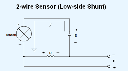
Okay, this can get confusing for first-time  4-20 mA current loop users. Yes, it is possible  to both power the sensor and measure the current it draws over the same two wires. In the 2-wire examples shown here, only two wires connect the sensor to its power supply, and the sensor draws current from it in direct proportion to the mechanical property that it measures. As current changes, the voltage developed across resistor R will change, thus providing a signal that’s suitable to connect to a measuring instrument like a data logger or data acquisition system.

In most situations, care should be taken to place the resistor in the low-side of the loop as shown here, as opposed to the high-side. Doing so will allow non-isolated instruments to make the measurement. In the next section, I’ll deal with a high-side shunt placement and discuss these cautions in more detail.

2-wire Sensors (High-side Shunt)

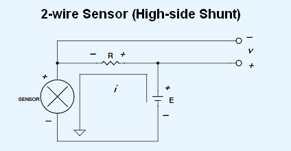
This configuration is almost exactly like the low-side, 2-wire approach, but it places the shunt resistor in the high-side of the loop. Note that while the voltage across the resistor is proportional to the current drawn by the sensor (just like the low-side approach), there is also a common mode voltage (CMV) present on either side to ground. On one side to ground the CMV is equal to the supply voltage. On the other side to ground it’s equal to the supply voltage, less the voltage dropped by the resistor (v). The presence of the CMVs places conditions on the instrument that you use to measure v. Specially, the instrument needs to have an isolated front end so it can float to the level of the CMV and still successfully make the measurement. Try this with a non-isolated, single-ended instrument and you will short-circuit the sensor to ground. A non-isolated differential instrument will either saturate or provide erroneous results.

3-wire Sensors

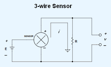
Three-wire sensors with a process current output have a separate wire for ground, signal (4-20 mA), and the power supply. This configuration is the easiest for current loop beginners to grasp, one input for power and a second for the current loop with a common ground. The primary advantage of a 3-wire sensor over its 2-wire counterpart is its ability to drive higher resistive loads. Resistors drop voltage for any given current in direct proportion to their resistance value. Holding current constant, higher resistances drop more voltage. Turning back to the 2-wire sensor and holding current constant, as the shunt resistance increases the voltage drop across the sensor also increases. You might reach a point where the voltage dropped by the shunt lowers the voltage drop across the sensor below the minimum required for it to operate properly.

We had a customer whose 2-wire current loop measurements functioned beautifully until loop current reached about 18 mA, at which point everything went  haywire. Upon close examination, we determined that the supply voltage she used was too low by at least 0.56-V. She needed 2 mA more measurement to reach full scale, which translates to 0.56 V with her 250-Ohm resistor. The solution was to use a higher voltage power supply to ensure that the voltage drop across the sensor stayed above the minimum level. She could have also used a 3-wire sensor, which ensures that the voltage applied to the sensor is independent of shunt resistor voltage drop.

Watch Your Grounds (or use an isolated instrument)

Contrary to what many believe (and have been erroneously taught in school), grounds are almost never the same in industrial settings, exactly where most 4-20 mA current loop sensors are used. Two or more grounds that are the same means that they are at the same potential. If so, a measurement between the grounds of the various field sensors and the instrument using a digital volt meter (DVM) on both its DC and AC settings will show zero volts, or very close to it. In reality, you’ll measure at least several volts, and I’ve seen as much as 75 Volts. When grounds that are not at the same potential are tied together (which you need to do to make the measurement), current flows through them, creating several possible measurement outcomes for non-isolated instruments:

1. The measurement is noisy.
2. The measurement is inaccurate.
3. You irreparably damage the instrument.
4. You saturate the instrument (it’s not damaged, but you can’t make a successful measurement, either.)

To remedy these problems requires the following:

1. Use an isolated instrument for your 4-20 mA current loop measurements. This single decision allows you to ignore all other grounding issues in exchange for successful measurements in any situation. If you don’t have an isolated instrument, read on…
2. Ensure that the loop power source is isolated. This means that its output ground (the one connected to the sensor) is not tied to its input ground (the one that connects to AC line power.) An isolated power source means that the output ground can be tied to another ground (like a non-isolated instrument) without consequence.
3. In self-powered applications, ensure that the low-side of the loop is isolated from its power source.
4. If you lack control over the power sources and determine that they are not isolated, then your only option is to power ALL devices (power supplies, self-powered sensors, the instrument, and its connected PC) from exactly the same power outlet. Don’t make the mistake of using outlets that are close to each other. If you run out of receptacles on a single outlet, then use a power strip.

Again, it’s worth repeating that all of the cautions associated with proper grounding disappear if an isolated instrument is used to make the measurement.

Sensors with 4-20 mA outputs are encountered in all disciplines and in many configurations.

Architecture of PLC- Part 1

    PLC system contains of the following parts

• Power supply
• CPU 
• Input modules
• Output modules
• Programming Device

Power Supply:

 This module supplies power to the CPU, input and output modules. It can be built into the PLC or be an external unit. Common voltage levels required by the PLC (with and without the power supply) are

24Vdc, 120Vac, 220Vac.

CPU (Central Processing Unit):

This module is considered as the brain of the PLC system and where 

ladder logic is stored and processed.

•The memory contains the data and the ladder program.

It contains an “Executive” program that tells the PLC how to:

• Execute the control Instructions

• User’s Program

• Communicate with other devices

• Other PLCs, Programming devices, I/O devices, etc.

• Perform Housekeeping activities

• Diagnostics, etc

This program is stored in “nonvolatile” memory

• Meaning that the program will not be lost if power is removed.